“Arbitrage is the practice of taking advantage of a price difference between two or more markets”
1 Theoretical Foundation
Arbitrage represents one of the fundamental concepts in financial markets, describing the simultaneous purchase and sale of identical or equivalent assets in different markets to profit from price discrepancies. In cryptocurrency markets, this principle applies to the price variations observed across different exchanges for the same digital asset.
As demonstrated in our price analysis, cryptocurrency exchanges do not always maintain identical prices for the same asset. These market inefficiencies create opportunities for risk-free profit through systematic arbitrage strategies.
Classical Arbitrage Example:
Consider the following scenario involving Ethereum trading:
- Step 1: Ethereum trades at €700 on Kraken Exchange
- Step 2: Simultaneously, Ethereum trades at €750 on
Bitstamp Exchange
- Step 3: Purchase 1 ETH on Kraken for €700
- Step 4: Transfer the ETH to Bitstamp
- Step 5: Sell 1 ETH on Bitstamp for €750
- Result: €50 profit (7.1% return) with theoretically zero market risk
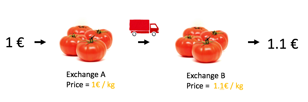
Conceptual Illustration: The following diagram illustrates the arbitrage principle using a simplified commodity example - purchasing tomatoes at €1.00/kg and selling at €1.10/kg. The same fundamental principle applies to cryptocurrency arbitrage, but with instantaneous execution and digital asset transfers.
2 Market Constraints and Limitations
While the theoretical arbitrage model appears straightforward, real-world implementation encounters several significant constraints that impact profitability and feasibility:
2.1 Economic Constraints
- Price Difference Frequency: As quantified in our analysis, significant price discrepancies (>1%) occur only 200-400 times daily per currency pair
- Transaction Costs: Each buy/sell operation incurs fees, typically 0.25% per transaction on most exchanges
- Spread Costs: The bid-ask spread creates additional costs beyond stated transaction fees
- Minimum Trade Sizes: Exchanges impose minimum order values that may limit small-scale arbitrage
2.2 Technical Constraints
- Market Velocity: Price discrepancies often disappear within seconds, requiring automated execution systems
- Slippage Risk: Order execution at different prices than expected due to market movement
- Transfer Delays: Cryptocurrency transfers between exchanges can take minutes to hours
- API Limitations: Rate limits and latency in exchange APIs affect execution speed
2.3 Operational Constraints
- Capital Concentration Risk: Successful arbitrage may concentrate funds in consistently expensive exchanges
- Liquidity Constraints: Large orders may impact market prices, reducing arbitrage margins
- Regulatory Risk: Varying regulations across exchanges and jurisdictions
- Counterparty Risk: Exchange insolvency or operational failures
2.4 Market Risk Factors
- Volatility Exposure: Holding cryptocurrency during transfer periods exposes capital to price volatility
- Correlation Risk: Market-wide movements can eliminate arbitrage opportunities
- Execution Risk: Technical failures during critical trading moments
3 Advanced Arbitrage Strategy: Paired Trading
To mitigate the transfer delay problem and reduce volatility exposure, sophisticated arbitrage strategies employ simultaneous paired trading across exchanges without physical asset transfers.
Enhanced Strategy Framework:
- Phase 1: Identify price discrepancy (Exchange A < Exchange B)
- Phase 2: Simultaneously execute:
- Buy cryptocurrency on Exchange A (lower price)
- Sell equivalent amount on Exchange B (higher price)
- Phase 3: Monitor for reverse price discrepancy
(Exchange A > Exchange B)
- Phase 4: Execute reverse trades:
- Sell on Exchange A
- Buy on Exchange B
- Result: Profit from both directions while maintaining market-neutral position
library(tidyverse)
library(gganimate)
library(tweenr)

# Initialize portfolio simulation data
initial_state <- data.frame(
  x = c(1,4,1,4),
  y = c(3,3,1,1),
  value = rep(100, 4),
  total_fiat = rep(200,4),
  total_crypto = rep(200,4),
  arrow1 = rep(0,4),
  arrow2 = rep(0,4),
  arrow3 = rep(0,4),
  arrow4 = rep(0,4)
)

# Define trading functions for simulation
execute_trade_1 <- function(portfolio){
  trade_amount = 50
  profit_margin = 1.8
  portfolio$value[1] <- portfolio$value[1] - trade_amount
  portfolio$value[2] <- portfolio$value[2] + trade_amount
  portfolio$total_fiat <- portfolio$value[1] + portfolio$value[3]
  portfolio$total_crypto <- portfolio$value[2] + portfolio$value[4]
  portfolio$arrow1 <- 1
  portfolio$arrow2 <- 0
  portfolio$arrow3 <- 0
  portfolio$arrow4 <- 0
  return(portfolio)
}

execute_trade_1_complete <- function(portfolio){
  trade_amount = 50
  profit_margin = 1.8
  portfolio$value[3] <- portfolio$value[3] + trade_amount * profit_margin
  portfolio$value[4] <- portfolio$value[4] - trade_amount
  portfolio$total_fiat <- portfolio$value[1] + portfolio$value[3]
  portfolio$total_crypto <- portfolio$value[2] + portfolio$value[4]
  portfolio$arrow1 <- 0
  portfolio$arrow2 <- 1
  portfolio$arrow3 <- 0
  portfolio$arrow4 <- 0
  return(portfolio)
}

execute_trade_2 <- function(portfolio){
  trade_amount = 50
  profit_margin = 1.8
  portfolio$value[3] <- portfolio$value[3] - trade_amount
  portfolio$value[4] <- portfolio$value[4] + trade_amount
  portfolio$total_fiat <- portfolio$value[1] + portfolio$value[3]
  portfolio$total_crypto <- portfolio$value[2] + portfolio$value[4]
  portfolio$arrow1 <- 0
  portfolio$arrow2 <- 0
  portfolio$arrow3 <- 1
  portfolio$arrow4 <- 0
  return(portfolio)
}

execute_trade_2_complete <- function(portfolio){
  trade_amount = 50
  profit_margin = 1.8
  portfolio$value[1] <- portfolio$value[1] + trade_amount * profit_margin
  portfolio$value[2] <- portfolio$value[2] - trade_amount
  portfolio$total_fiat <- portfolio$value[1] + portfolio$value[3]
  portfolio$total_crypto <- portfolio$value[2] + portfolio$value[4]
  portfolio$arrow1 <- 0
  portfolio$arrow2 <- 0
  portfolio$arrow3 <- 0
  portfolio$arrow4 <- 1
  return(portfolio)
}

# Execute trading simulation sequence
trading_sequence <- list(initial_state, initial_state, initial_state)
current_portfolio <- initial_state
sequence_step <- 1

# Simulate one complete arbitrage cycle
for(cycle in 1){
  # Execute first trade pair
  sequence_step <- sequence_step + 1
  current_portfolio <- execute_trade_1(current_portfolio)
  trading_sequence[[sequence_step]] <- current_portfolio

  # Complete first trade
  sequence_step <- sequence_step + 1
  current_portfolio <- execute_trade_1_complete(current_portfolio)
  trading_sequence[[sequence_step]] <- current_portfolio

  # Execute reverse trade pair
  sequence_step <- sequence_step + 1
  current_portfolio <- execute_trade_2(current_portfolio)
  trading_sequence[[sequence_step]] <- current_portfolio

  # Complete reverse trade
  sequence_step <- sequence_step + 1
  current_portfolio <- execute_trade_2_complete(current_portfolio)
  trading_sequence[[sequence_step]] <- current_portfolio
}

# Create smooth animation transitions
animated_data <- tween_states(trading_sequence, tweenlength = 0.01, statelength = 0.1,
                             ease = c('cubic-in-out'), nframes = 100)

# Generate arbitrage visualization
arbitrage_plot <- animated_data %>%
  ggplot(aes(x=x, y=y, size=value, frame=.frame)) +
  theme_void() +
  geom_point(aes(color=paste(x,y))) +
  scale_color_manual(values=c("#69b3a2", "purple", "#69b3a2", "purple")) +
  scale_size_continuous(range=c(1,30)) +
  theme(legend.position="none") +

  # Portfolio values display
  geom_text(aes(label=round(value,0), x=x, y=y-0.5, color=paste(x,y)), size=6) +

  # Exchange labels
  geom_label(x=-1, y=3, label="Exchange 1", color="purple", size=5) +
  geom_label(x=-1, y=1, label="Exchange 2", color="#69b3a2", size=5) +

  # Trading arrows
  geom_segment(aes(alpha=arrow1), x=1.8, xend=3.2, y=3, yend=3, size = 1,
               arrow = arrow(length = unit(0.5, "cm"))) +
  geom_segment(aes(alpha=arrow2), x=3.2, xend=1.8, y=1, yend=1, size = 1,
               arrow = arrow(length = unit(0.5, "cm"))) +
  geom_segment(aes(alpha=arrow3), x=1.8, xend=3.2, y=1, yend=1, size = 1,
               arrow = arrow(length = unit(0.5, "cm"))) +
  geom_segment(aes(alpha=arrow4), x=3.2, xend=1.8, y=3, yend=3, size = 1,
               arrow = arrow(length = unit(0.5, "cm"))) +

  # Alpha control for arrows
  scale_alpha_continuous(range=c(0,1)) +

  # Portfolio total bars
  geom_segment(x=1, xend=1, y=-1, aes(yend=(0-(-0.8)/(500-200))*total_fiat-1.33),
               color="yellow", size=22, alpha=0.7) +
  geom_segment(x=4, xend=4, y=-1, aes(yend=(0-(-0.8)/(500-200))*total_crypto-1.33),
               color="yellow", size=22, alpha=0.7) +

  # Portfolio labels
  geom_text(x=1, y=-.5, label="Total Fiat", color="grey", size=5) +
  geom_text(x=4, y=-.5, label="Total Crypto", color="grey", size=5) +
  geom_text(x=1, y=-.8, aes(label=round(total_fiat,0)), color="grey", size=5) +
  geom_text(x=4, y=-.8, aes(label=round(total_crypto,0)), color="grey", size=5) +

  # Asset type labels
  geom_label(x=1, y=4, label="Fiat Currency", color="black", size=5) +
  geom_label(x=4, y=4, label="Cryptocurrency", color="black", size=5) +

  # Title and subtitle
  ggtitle("Paired Arbitrage Strategy Simulation") +
  theme(plot.title = element_text(size=16, hjust=0.5, color="grey"))

arbitrage_plot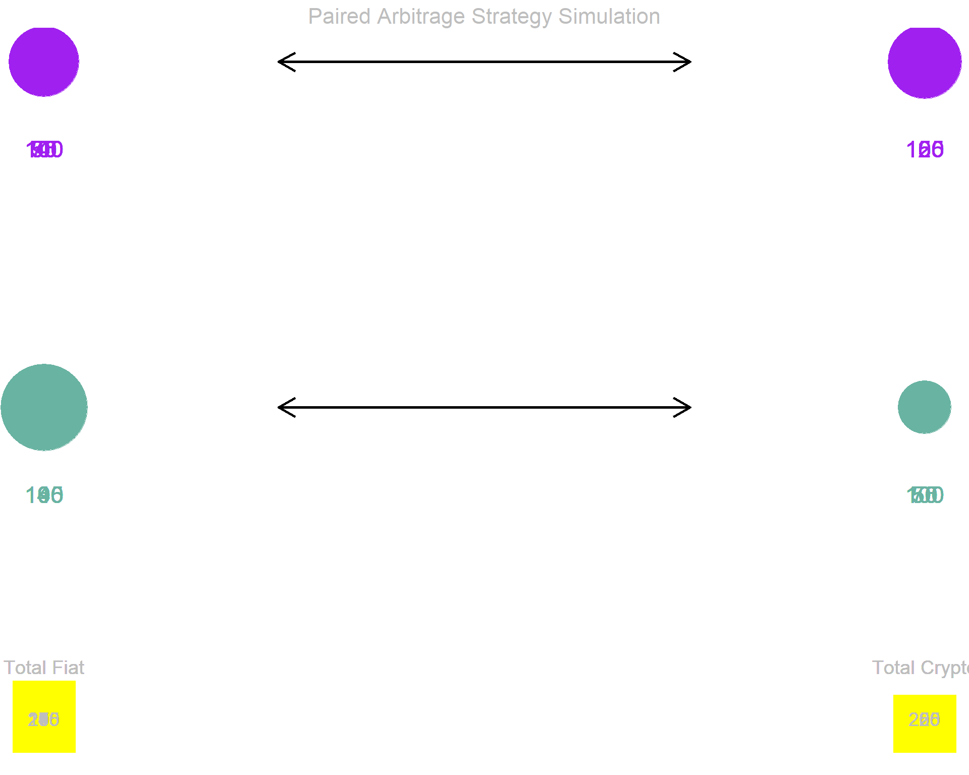
Strategic Advantages:
- Eliminates Transfer Risk: No cryptocurrency transfers between exchanges
- Reduces Volatility Exposure: Market-neutral
position during holding periods
- Faster Execution: No waiting for blockchain confirmations
- Capital Efficiency: Profits from both directional price movements
- Scalability: Can be applied across multiple exchange pairs simultaneously
4 Risk Management Framework
Successful arbitrage implementation requires comprehensive risk management addressing both systematic and operational risks:
4.1 Capital Allocation Strategy
- Diversification: Spread capital across multiple exchange pairs
- Position Sizing: Limit individual trade size to manage impact costs
- Reserve Management: Maintain adequate reserves for rebalancing
4.2 Technical Risk Controls
- Automated Monitoring: Real-time price difference detection
- Execution Limits: Maximum acceptable slippage thresholds
- Failsafe Mechanisms: Automatic position closure on technical failures
4.3 Market Risk Mitigation
- Volatility Filters: Suspend trading during high volatility periods
- Correlation Monitoring: Track inter-exchange price relationships
- Liquidity Assessment: Ensure adequate market depth before execution
5 Implementation Roadmap
The theoretical framework established here provides the foundation for practical arbitrage implementation. The next phase involves developing automated trading systems capable of executing these strategies at the speed and scale required for profitability.
Key implementation components include:
- Real-time Market Data Integration
- Automated Decision Algorithms
- High-Speed Order Execution Systems
- Risk Management Protocols
- Performance Monitoring and Optimization